Using spatial resamples for analysis

The resampled objects created by spatialsample can be used in many of the same ways that those created by rsample can, from making comparisons to evaluating models. These objects can be used together with other parts of the tidymodels framework, but let’s walk through a more basic example using linear modeling of housing data from Ames, IA.

data("ames", package = "modeldata")

The Ames housing data is a normal tibble. While many of the functions in spatialsample support standard tibbles, several require that our data be an sf object to properly handle spatial distance calculations. We can transform our Ames data into an sf object using the sf::st_as_sf() function:

ames_sf <- sf::st_as_sf(
  ames,
  # "coords" is in x/y order -- so longitude goes first!
  coords = c("Longitude", "Latitude"),
  # Set our coordinate reference system to EPSG:4326,
  # the standard WGS84 geodetic coordinate reference system
  crs = 4326
)

For this vignette, we’ll model the sale prices of the houses in the Ames data set. Let’s say that the sale price of these houses depends on the year they were built, their living area (size), and the type of house they are (duplex vs. townhouse vs. single family), along with perhaps interactions between type and house size.

log10(Sale_Price) ~ Year_Built + Gr_Liv_Area + Bldg_Type

This relationship may exhibit spatial autocorrelation across the city of Ames, and we can use any of the several different methods provided by spatialsample to try and investigate it.

For instance, we could create v = 15 spatial cross-validation folds with spatial_clustering_cv(), which uses k-means clustering in order to divide the data into folds. We can then visualize those folds using the autoplot() function from spatialsample:

library(spatialsample)

set.seed(123)
cluster_folds <- spatial_clustering_cv(ames_sf, v = 15)

autoplot(cluster_folds)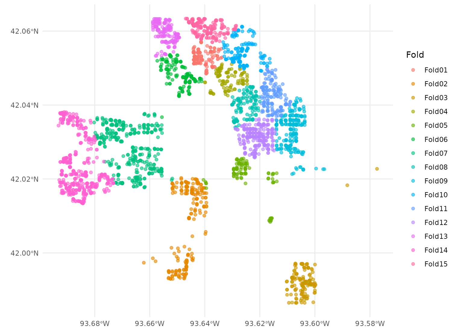

Our cluster_folds object is an rset object that contains many resamples or rsplit objects in the splits column. The resulting partitions do not necessarily contain an equal number of observations:

cluster_folds
#> #  15-fold spatial cross-validation 
#> # A tibble: 15 × 2
#>    splits             id    
#>    <list>             <chr> 
#>  1 <split [2797/133]> Fold01
#>  2 <split [2724/206]> Fold02
#>  3 <split [2777/153]> Fold03
#>  4 <split [2830/100]> Fold04
#>  5 <split [2836/94]>  Fold05
#>  6 <split [2759/171]> Fold06
#>  7 <split [2560/370]> Fold07
#>  8 <split [2810/120]> Fold08
#>  9 <split [2715/215]> Fold09
#> 10 <split [2776/154]> Fold10
#> 11 <split [2778/152]> Fold11
#> 12 <split [2695/235]> Fold12
#> 13 <split [2750/180]> Fold13
#> 14 <split [2496/434]> Fold14
#> 15 <split [2717/213]> Fold15

But while spatial clustering is a method for spatial cross-validation using spatialsample, it is not the only method available. The other methods are broadly similar, breaking the data into a number of (not necessarily even) folds based on spatial arrangement.

For instance, the spatial_block_cv() function will perform spatial blocking with your data:

set.seed(123)
block_folds <- spatial_block_cv(ames_sf, v = 15)

autoplot(block_folds)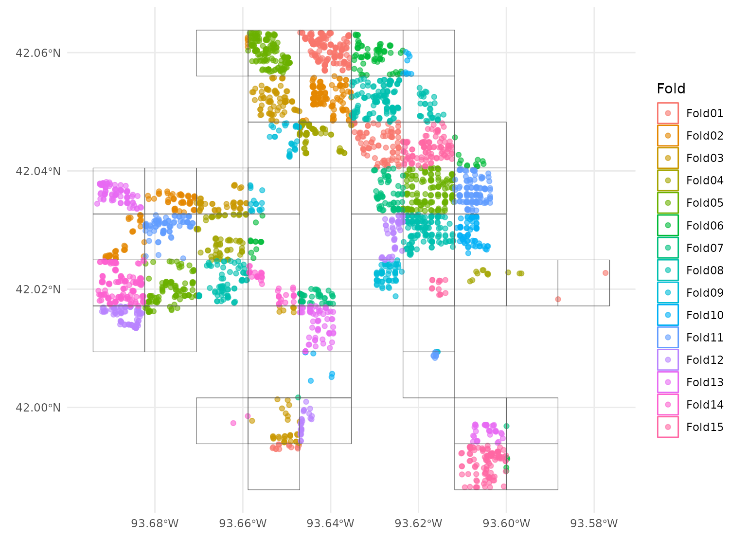

If you already have a sense of what locations in your data are likely to be closely related, you can also use the spatial_leave_location_out_cv() function to perform leave-location-out cross-validation. For instance, we can split the Ames data into folds based on neighborhoods using this function:

set.seed(123)
location_folds <-
  spatial_leave_location_out_cv(
    ames_sf,
    group = Neighborhood,
    v = 15
  )

autoplot(location_folds)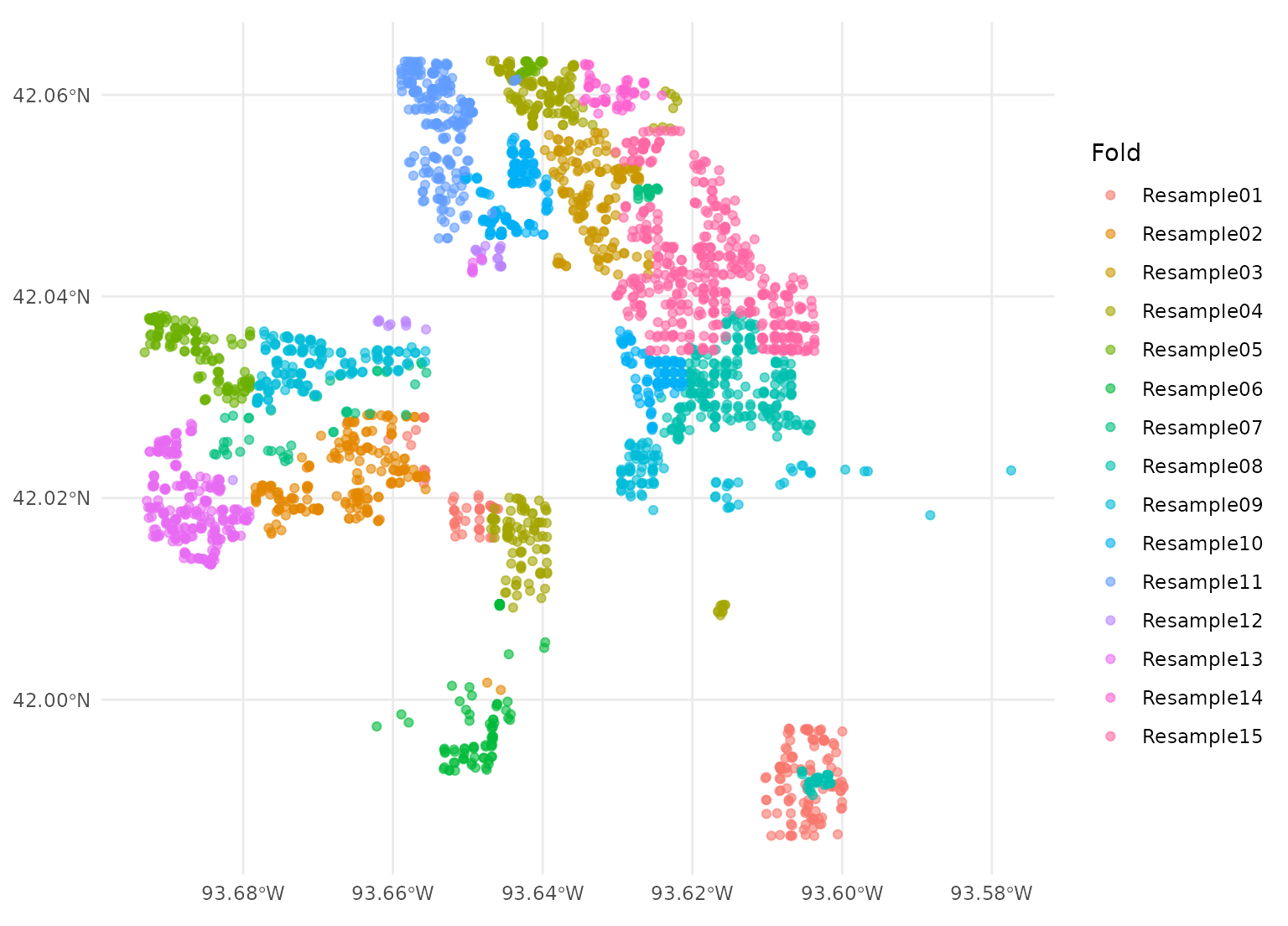

We’ve now got a lot of different resamples floating around! We’re going to fit the same models to each of them, in the same way, using the same code. In order to make that task a little easier, let’s add a new column named type to signal what type of resample each fold is from, and then combine them into a new data frame:

cluster_folds$type <- "cluster"
block_folds$type <- "block"
location_folds$type <- "location"

resamples <-
  dplyr::bind_rows(
    cluster_folds,
    block_folds,
    location_folds
  )

Now let’s write a function that will, for each resample:

• obtain the analysis set for model fitting
• fit a linear model with a interaction term
• predict the assessment set and return both the true and predicted price, on the log scale

# `splits` will be the `rsplit` object
compute_preds <- function(splits) {
  # fit the model to the analysis set
  mod <- lm(log10(Sale_Price) ~ Year_Built + Bldg_Type * log10(Gr_Liv_Area),
    data = analysis(splits)
  )
  # identify the assessment set
  holdout <- assessment(splits)
  # return the assessment set, with true and predicted price
  tibble::tibble(
    geometry = holdout$geometry,
    Sale_Price = log10(holdout$Sale_Price),
    .pred = predict(mod, holdout)
  )
}

We can apply this function to just one of the splits.

compute_preds(cluster_folds$splits[[7]])
#> # A tibble: 370 × 3
#>                geometry Sale_Price .pred
#>             <POINT [°]>      <dbl> <dbl>
#>  1 (-93.67907 42.03608)       4.83  4.99
#>  2 (-93.67721 42.03654)       5.05  5.20
#>  3 (-93.67367 42.03479)       5.17  5.14
#>  4 (-93.67096 42.03569)       5.14  5.06
#>  5  (-93.6721 42.03486)       5.09  5.07
#>  6 (-93.67207 42.03457)       5.12  5.11
#>  7 (-93.66969 42.03533)       5.10  5.10
#>  8  (-93.66067 42.0346)       5.23  5.25
#>  9 (-93.65921 42.03456)       5.12  5.26
#> 10 (-93.65623 42.03345)       5.39  5.33
#> # ℹ 360 more rows

Or we can apply this function to all of the splits, using purrr::map().

library(purrr)
library(dplyr)
#> 
#> Attaching package: 'dplyr'
#> The following objects are masked from 'package:stats':
#> 
#>     filter, lag
#> The following objects are masked from 'package:base':
#> 
#>     intersect, setdiff, setequal, union

cv_res <- resamples %>%
  mutate(.preds = map(splits, compute_preds))

We can unnest() these results and use yardstick to compute any regression metrics appropriate to this modeling analysis, such as yardstick::rmse():

library(tidyr)
library(yardstick)

cv_rmse <- cv_res %>%
  unnest(.preds) %>%
  group_by(id, type) %>%
  rmse(Sale_Price, .pred)

cv_rmse
#> # A tibble: 45 × 5
#>    id     type    .metric .estimator .estimate
#>    <chr>  <chr>   <chr>   <chr>          <dbl>
#>  1 Fold01 block   rmse    standard      0.0788
#>  2 Fold01 cluster rmse    standard      0.0715
#>  3 Fold02 block   rmse    standard      0.0705
#>  4 Fold02 cluster rmse    standard      0.104 
#>  5 Fold03 block   rmse    standard      0.0757
#>  6 Fold03 cluster rmse    standard      0.107 
#>  7 Fold04 block   rmse    standard      0.0962
#>  8 Fold04 cluster rmse    standard      0.0542
#>  9 Fold05 block   rmse    standard      0.103 
#> 10 Fold05 cluster rmse    standard      0.146 
#> # ℹ 35 more rows

It looks like the RMSE may vary across the city, so we can join the metrics back up to our results and plot them.

library(ggplot2)

cv_res %>%
  unnest(.preds) %>%
  left_join(cv_rmse, by = c("id", "type")) %>%
  ggplot(aes(color = .estimate)) +
  geom_sf(aes(geometry = geometry), alpha = 0.5) +
  labs(color = "RMSE") +
  scale_color_viridis_c() +
  facet_wrap(vars(type), ncol = 1)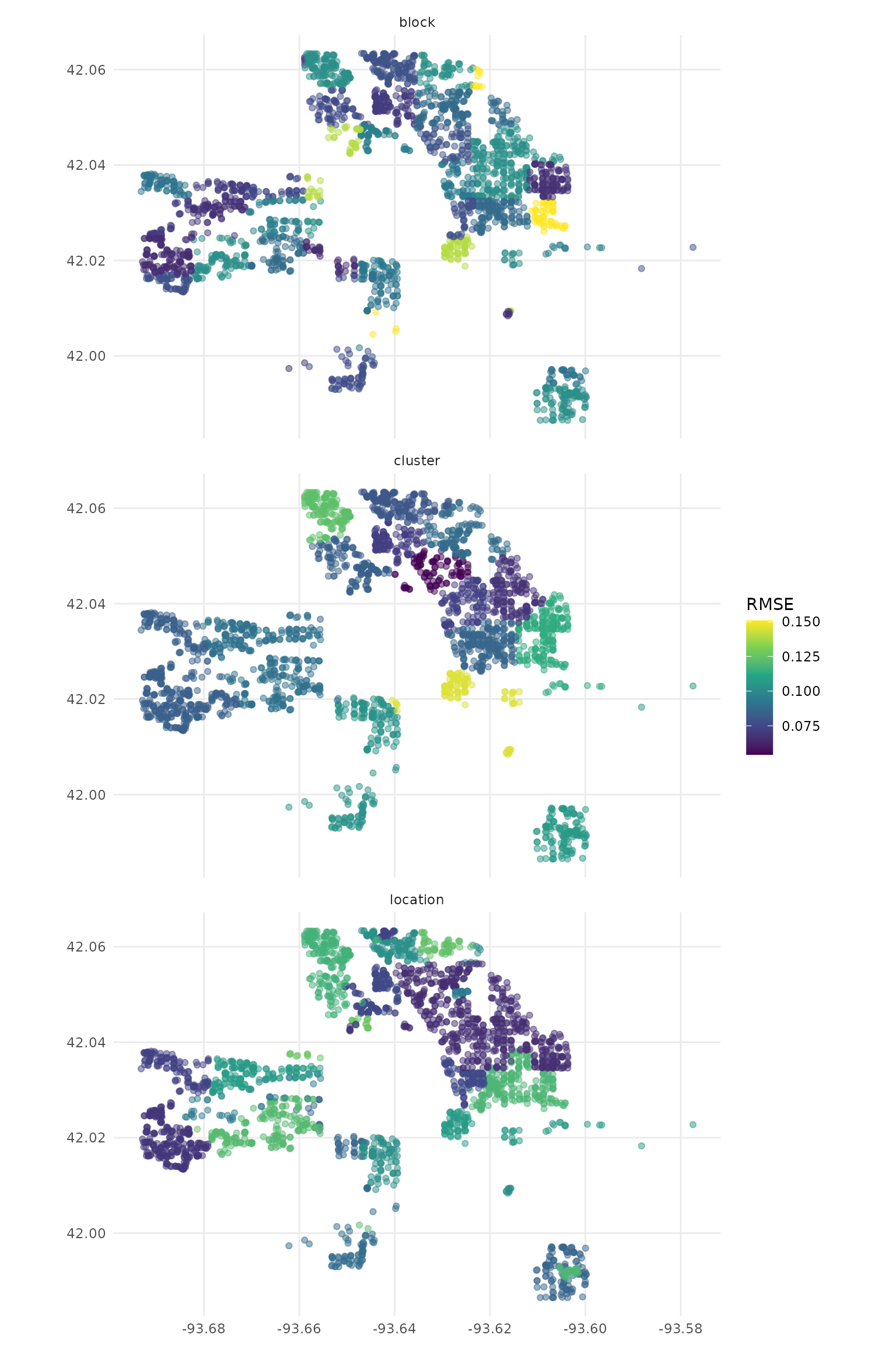

As you can see, the results you get are highly dependent on how you resample your data! It’s important to use the right method for your data (and, for methods like spatial blocking and buffered cross-validation, the right distances).